Introduction

Recently, I have been working on a project that dealt with large sets of latency measurements. For these, I always needed to capture percentile values (e.g., p50, p95, p99, etc.). Since I was working with SQLite, I naturally used the stats extension to calculate those percentiles, which worked OK until it didn’t! I realized that the single percentile calculation required a surprisingly consistent ~3ms for every 10K rows of data. This meant it was totally unsuitable for data sets in the 10s or 100s of millions in size, far off the performance targets of the application in question. So what’s next?

Finding Alternatives

Another statistical SQLite extension?

I first started looking at what other statistical extensions exist for SQLite, but nothing came out as useful for my performance requirements. There are some interesting data structures out there, like Q-Digest, T-Digest & KDD-Sketches. These offer hugely better performance and usually acceptable accuracy for quantile estimation. But none were available as a SQLite extension.

Another Embedded Database?

Then, I thought I would consider DuckDB, the other embedded db that is built entirely on being a super analytical power house. And indeed, DuckDB was fast, around 25X faster than SQLite! Now dealing with 10s of millions of rows seems feasible, but probably 100s of millions or billions are out of the questions. Also, DuckDB had a major drawback: you cannot connect to it from multiple processes unless all connections are read only. Given the nature of the application, this meant that a huge amount of work was required to enable live data introspection and debugging.

You might be asking, though, “Why am I stuck with an embedded database?” Well, that’s due to the nature of the application, so it’s a limitation we are living with.

Roll my own solution?

I kept that option last, since I was trying to optimize for developer time. And even when I entertained that option I was thinking of building a SQLite extension around an existing implementation of one of the data structures listed above. But I struggled with getting T-Digest to work, so I thought, well, let me take a stab at building something simpler and see how it goes.

Defining The Requirements

The quantile calculations are generally slow because they need the sort through a large set of data elements and return the item at a specific point. E.g., calculating p90 of a 1M unsorted array requires sorting the array and then counting 100K of the elements from largest to smallest and returning the element at index 100K from max. This is generally expensive because of the need to scan and sort the data in memory. The same is true if you are trying to filter this data by other columns in the table, which could make the sorting step faster, but the scan remains problematic.

Thus in became clear that we wanted to implement a summary data structure in the spirit of Q-Digest or T-Digest, with this list of requirements:

High performance quantile queries

Naturally, since this whole effort is about bringing forth efficient percentile calculations. Getting it to work well was not enough; it had to be very fast.

Small size in general, specially so when serialized

Summary data structures cannot be sliced and diced, hence we might need to store many of them to cover the dimensions we need to report at and their permutations. A small serialized size is critical to make this possible.

Can merge multiple data structures, fast

If we have data spread out across many dimensions and dimension values, then if it can be merged together we can skip having to store aggregations of this data and perform these queries on the fly. Allowing us to simplify our storage mode.

Works well in a database environment

A database centric workflow means data is most of the time is stored in tables in a serialized format. It will be greatly beneficial if we can reduce the serialize/deserialize overhead or eliminate it completely whenever possible

With defined error bounds

We need to have a certain level of confidence in the data we are reporting. If a certain percentile query is very fast but is off by 20% then it is not really useful.

Easy to reason about and maintain

A simple foundation is easier to prove correct and build on top of it later. Ideas like on-the-fly lookup tables, index bitmaps, FMA math and min-max index were pushed back to keep the design as simple as possible at the beginning at least. The target was a portable, small library that could fit in a single header file with zero dependencies.

The Data Structure

The data structure itself is very simple, it is basically a histogram (hence the name Heistogram) with an array of buckets, containing the count of the values stored in that bucket.

typedef struct {
    uint64_t count;
} Bucket;

typedef struct {
    uint16_t capacity;       // Current capacity of buckets array
    uint16_t min_bucket_id;  // Smallest bucket id, for optimizing serialization
    uint64_t total_count;    // Total count of all values
    uint64_t min;            // Minimum value
    uint64_t max;            // Maximum value
    Bucket* buckets;         // Array of buckets, index = bucket ID
} Heistogram;

To perform a percentile query, you basically calculate the position you want to target as a fraction of the total count. Then you traverse the buckets in order accumulating the sum of their counts. You do this until the sum is equal to or exceed the value you calculated. At this point, you have hit the desired bucket. You calculate the bucket boundaries and do linear interpolation to get the desired value.

To make sure this is efficient, we use logarithmically growing bucket sizes. Ensuring that of any given bucket, the max value is larger than the min value by a fixed ratio, which is the max potential error margin for quantile queries. Value to bucket mapping is done according to the following formula:

bucket_id = floor(log2(value)/log2(1 + error_margin));

The current implementation is very thin on individual bucket data, just the count. But at the same time it can contain empty gap buckets. There are ways to potentially even optimize this further in the future but as it stands, it is already quite space efficient.

Optimizations

A few easy wins were achieved without too much investment in optimization, examples include:

• Pre-calculating the log value of the error margin to speed up bucket mapping
• Accepting gaps in the structure meant bucket ids were implicitly present
• Implicit bucket ids meant de-serializing didn’t require calculating bucket ids
• Percentile queries start at the end of the bucket array
• Variable length encoding is used for all integer values serialized
• Power calculations use a fast algorithm rather than relying on the pow() function

With these simple optimizations, on top of a simple and straightforward design the results was a really fast and tight histogram solution.

Database Specific Optimizations

Some optimizations were specific to making Heistogram integrate well withing a database environment, these include:

• Percentile queries can be performed directly on serialized data, without the need to deserialize
• Serialized data is laid out in a way to optimize for high percentile queries, e.g. p95, which are more common
• Aside from percentile queries, merge operations can also be performed directly on serialized Heistograms, without the need for deserialization.

Accuracy

As was mentioned, bucket sizes grow logarithmically, with each bucket size being equal the minimum value possible in the bucket * 1 + error_margin. Thus, for values large than 1/error_margin, the maximum possible error is well, error_margin! And this only happens when a bucket has entries that all happen to fall on one end of it (value wise) but the linear interpolation selects the value at the other end of the bucket.

To further illustrate that, here are some empirical test results on various data sets with different distributions. Tested here against DuckDB’s implementation of T-Digest

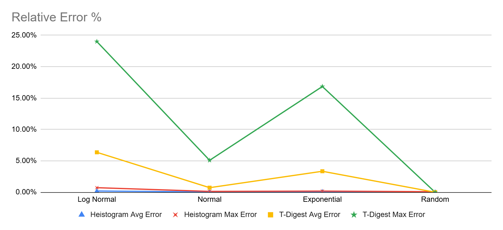
As can be seen, T-Digest maintains low error rates except for long-tail distributions (e.g., log-normal, Pareto or exponential) These results are influenced by p99.9, p99.99 and p99.999 values which had a large margin of error for the 13M value datasets with long tails. I am not sure though if that is a specific issue with DuckDB’s implementation of T-Digest

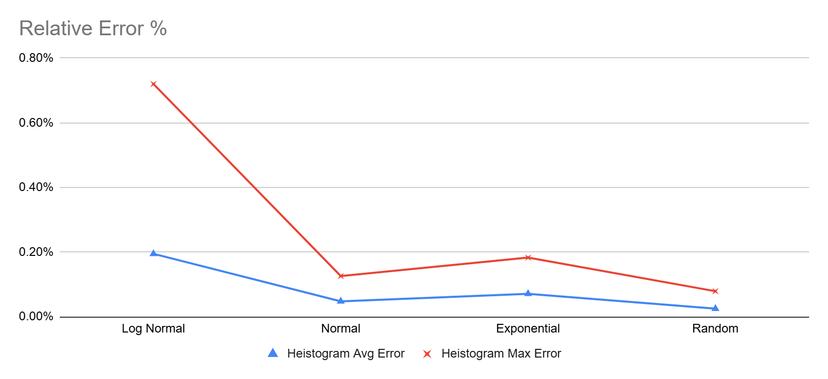
On the other hand Heistogram remained pretty accurate for all the tested percentile, the worst showing was 0.72% (that’s under 1%) error for the p99.999 value of the log-normal data set. Here’s another chart focusing only on Heistogram errors

I also started testing against reservoir percentile approximation, also available through DuckDB, but after a couple tries let me just say that this only works for uniform distributions. Don’t use it for latency data!

Performance

To test performance, I benchmarked certain operations and measured their average latencies. Since the operations are typically very fast, we had to resort to nano seconds to be able to show meaningful data

Insert Performance

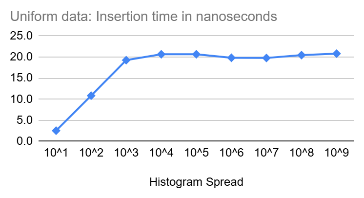
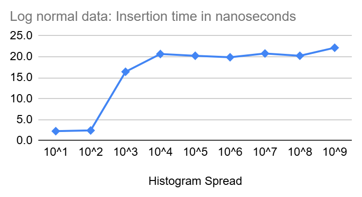
In the diagrams above, we see that inserts start at a few nano seconds for very tight Heistograms then climb quickly to settle around 20 nanoseconds for larger spread.

Percentile Query Performance

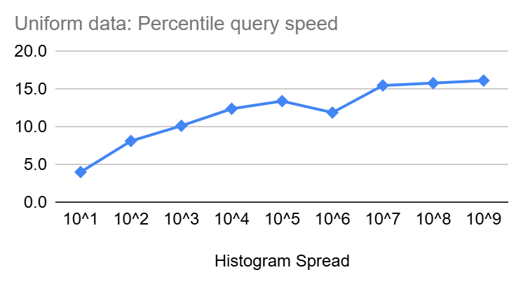
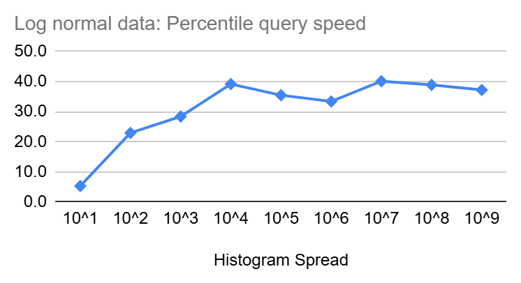
Similar to insertion speed, percentile queries start at a few nanoseconds but then increase slowly in size as the spread of the Heistogram increase until it reaches ~16ns and ~40ns for uniform and log-normal distributions, respectively, at a spread of 10^9. Though the increase is clearly sub-linear and should be increasing with even less steepness as we get closer to the end of the 64 Bit range.

Percentile Query Performance On Serialized Data

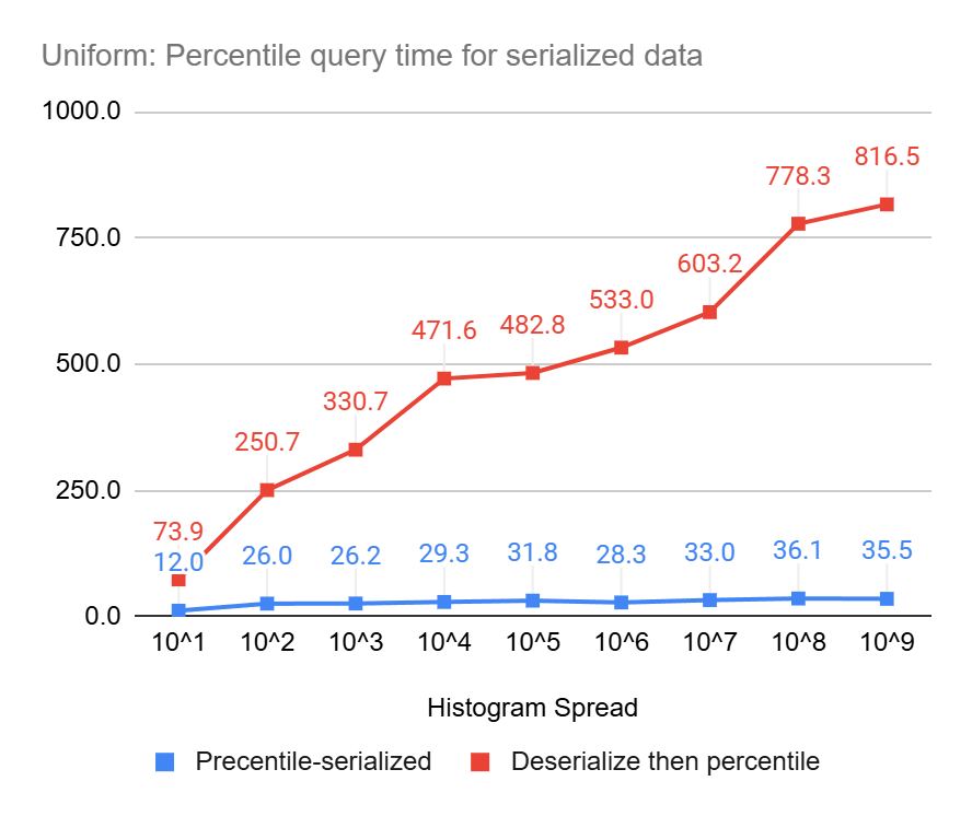
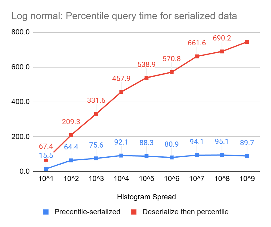
These charts clearly show the power of percentile queries on serialized data, compared to serializing first and then performing the queries, they end up being up to 23 times and 8 times faster, for uniform and log-normal data, respectively.

How Does It Compare to T-Digest?

We ran percentile & insert benchmarks from the C T-digest implementation provided by the Redis-Bloom project.

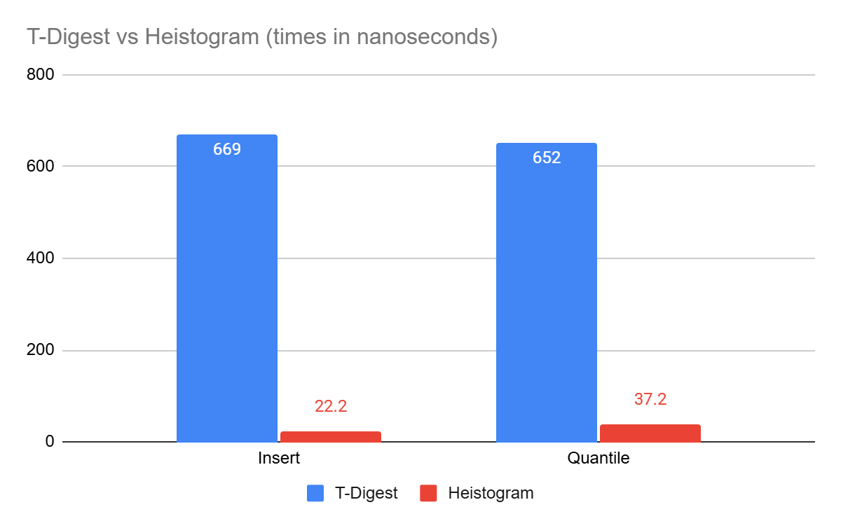
For typical operations, Heistogram is up to 20x faster than T-Digest on similar data sets (10M entries, log-normal distribution). Since Heistogram only supports integer values, the data spread for the test was chosen at 10^9.

Limitations

Heistogram can only store up to 2 ^ 64 – 1 values, all integers. The smallest possible value is 0 and the largest is also 2 ^ 64 – 1. If you need to store fractional data then you need to scale and round first.

If Heistogram contains all the values from 0 to 2 ^ 64 – 1, then it will serialize to ~18KB, this is an upper bound that cannot be exceed. Typcial sizes are much smaller.

Heistograms with data belonging to two overlapping data sets cannot be merged, as there will duplicates in the counts and wrong query results.

Conclusion

Finally I have a solution that meets the strict performance needs of the application I am working on. All the while being a fun little project that triggers my dopamine-inducing appetite for performance optimization and efficiency. I hope it would be useful to others as well. If you work with big data I sure hope you would give it a spin.

Since not everyone would happily be working directly with a C library, I am working on SQLite and Ruby bindings to make this easier to digest for as many developers/data engineers as possible. Contributions for ports to other languages/databases are more than welcome.

Please find the source code here