
Context
In this paper, titled “SQLite: Past, Present, and Future”, the SQLite core team, along with researchers from the University of Wisconsin-Madison discussed the progress timeline of SQLite, how it became a world class OLTP database engine, but also how it started to struggle with some of the emerging analytical workloads. Compared to DuckDB, an embedded database that build on a very similar philosophy to SQLite’s but with an OLAP focus, SQLite ended up trailing DuckDB for most analytical queries by a huge margin. In the paper, the authors discussed the possibility of using bloom filters to speed up some of these queries, and indeed, their efforts are fruitful and SQLite’s sees quite the performance jump in many analytical queries. Though that jump was not big enough to catch up with DuckDB, which still enjoyed a large lead over SQLite in the analytical domain.

But, an embedded database engine is not just about which query flavors is supports best. As someone who uses and maintains SQLite based apps a lot I can tell you that the flexibility of accessing the database for reading/writing from multiple processes is basically a must have in any development or production environment. Otherwise it will be virtually impossible to jump in and debug/observe the data state for a live application.
Not to mention that this feature results in SQLite being very easy to reason about its state. Allowing simpler and a lot more efficient backup schemes that don’t disrupt the running applications.
For these reasons I found it very hard to accept the idea of dropping SQLite for an other engine when I had an application that needed a lot of analytical queries. Mainly lots of percentile calculations. For that purpose, I built Heistogram, a C library for fast quantile estimation. I wrote about more in depth here.
In this post though, I want to talk about the SQLite wrapper I built for Heistogram so that I am able to run it from within SQLite. In the rest of this post, I will be talking about using Heistogram to speed up percentile queries over large data volumes in SQLites, and the different ways with which this can be achieved.
But SQLite is Fast Enough, NO?
Not for all types of queries. As we mentioned earlier, in some analytical queries SQLite will struggle to perform compared to other OLAP oriented engines like DuckDB
Consider the following scenario: You have a table with 13M entries of latency data, and you want to determine the following percentiles: p50, p95, p99
You can easily reach out the canonical stats extension (written by Dr. Richard Hipp himself) and type the following query in the SQLite console
SELECT
  percentile(sample, 99) AS p99
FROM
  samples;
Then you hit enter. Then you wait.
After around 4 seconds you will see the results appear on the screen. Now imagine you need to find these values for hundreds of customers that are using your application simultaneously. Not only is their experience horrible, 4 seconds to get a result, but they make every other online customer’s experience horrible as well. Since the system will struggle to keep up with all the load.
But why is it slow? It is because it has to load all 13M samples into memory and sort them before being able to get the percentile data. And yes, I know that using an index will speed that up considerably, but the storage requirements for that index (~145MB for that particular set) renders it infeasible due to the sheer amount of data sets that will need to be indexed.
Now let’s try to get 3 percentile values at once, your query will look something like this
SELECT
  percentile(sample, 50) AS p50,
  percentile(sample, 90) AS p90,
  percentile(sample, 99) AS p99
FROM
  samples;
That now takes over 9 seconds! Need more percentile data? 6 percentile points? 19 seconds to get what you need!
Now let’s fire up DuckDB to see how an OLAP optimized system deals with a similar request. We type the following in the DuckDB console:
SELECT
  quantile(sample, 0.99) AS p99
FROM
  samples;
Pretty similar, just some function name changes and percentiles in the range 0, 1 instead of 0, 100.
So now you press enter. And wait.
Not really, because the results were returned very fast, a little over a 100ms to be exact. How is that even possible? It is because DuckDB is columnar database, which uses min-max indexes that speed up queries like that by a lot and they take ~5% of the size of original column. The downside though is that the columns become disjoint and transactional operations will become much slower.
Like SQLite, query time increased linearly with the number of percentiles queried. Thus it maintained the huge over gap in relative performance.
To illustrate the huge difference in performance we performed percentile queries over a range of data distributions, 5 to be exact (random, normal, log normal, pareto & exponential). The we reported the average results of requesting 1, 3 and 6 percentile values from each distribution.
Here are the results in tabular format:
| Query time in seconds | 1 percentile query | 3 percentile queries | 6 percentile queries |
|---|---|---|---|
| SQLite | 3.74675 | 9.2577798 | 18.4866 |
| DuckDB | 0.1138 | 0.3734 | 0.7752 |
| DuckDB Advantage | 33X | 25X | 24X |
And in colored chart format:
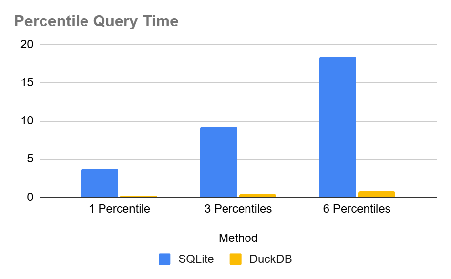
So, as it stands, DuckDB is almost 24x to 33x times faster than SQLite for this particular operation. But why don’t we try Heistogram to see if it can make a difference?
Take 1: Build a Heistogram on the fly
In this case, we will just query the original table like we did previously, but we will not use the percentile function, instead we will build a heistogram and pass it to an outer query that will calculate the percentiles
SELECT
  heist_percentile(h, 50) AS p50,
  heist_percentile(h, 95) AS p95,
  heist_percentile(h, 99) AS p99
FROM (
  SELECT
    heist_group_create(sample)
  FROM
    samples
);
When we press enter, this query comes back with the results in around 1.2 seconds, a huge improvement over the original query. And a quick jump to bridge the gap with the DuckDB engine. Similar results are achieved when tested against multiple data distributions. Here are the average run times in tabular format:
| Query time in seconds | 1 percentile query | 3 percentile queries | 6 percentile queries |
|---|---|---|---|
| SQLite | 3.74675 | 9.2577798 | 18.4866 |
| SQLite + Heistogram | 1.1944 | 1.1936 | 1.2022 |
| DuckDB | 0.1138 | 0.3734 | 0.7752 |
| DuckDB Advantage SQLite | 33X | 25X | 24X |
| DuckDB Advantege Heistogram | 10.5X | 3.2X | 1.6X |
And in chart format:
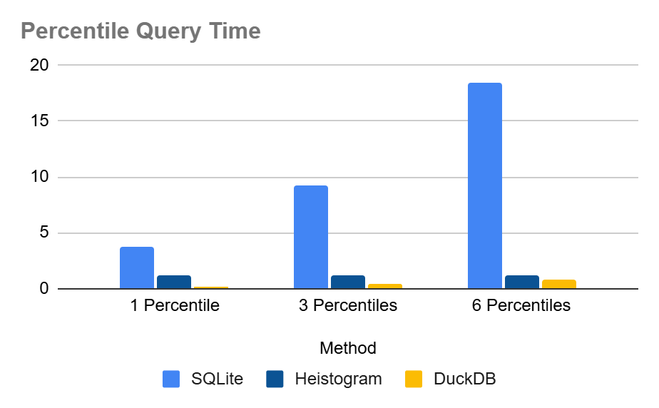
This is quite the improvement. Specially when we want to query a large amount of percentile values. Heistogram is almost constant time regardless of the number of queries. This is due to the benchmark being dominated by the time to pass through the data and create the heistogram in the first place. The 10s of nanoseconds for each percentile query are practically inconsequential.
In reality though, these number are not good enough for my application. Even the DuckDB numbers, as impressive they are, are nowhere good enough for our performance targets. Let’s see how can we improve this
Take 2: Persist and Query Serialized Heistogram(s)
Instead of creating heistograms on the fly, we can create them and persist them in a table. A sample schema could look like:
CREATE TABLE heistograms (
  id INTEGER PRIMARY KEY,
  h BLOB
);
Then we can populate it with our sample data as such
INSERT INTO
  heistograms
SELECT
  1,
  heist_group_create(sample)
FROM
  samples;
Before, running any percentiles queries, I am interested to see how big is the heistogram blob. Turns out it is 892 bytes. Such a small fraction of the original 34MB of the sample column
Now we run the percentiles query
SELECT
  heist_percentile(h, 50) AS p50,
  heist_percentile(h, 95) AS p95,
  heist_percentile(h, 99) AS p99
FROM
  heistograms
WHERE
  id = 1;
How fast does this run? Well the console says 0.0 seconds.
We try again, this time repeating the operation a 100 times, still 0.0. A 1000 times, still also 0.0. We increase the iterations until we discover it is performing (on average over the different distributions) over 1M iterations of this query in a second. I.e. it is reporting over 3M percentile values in a second!
| Query time in seconds | 1 percentile query | 3 percentile queries | 6 percentile queries |
|---|---|---|---|
| Heistogram Index | 0.0000002882 | 0.000001012 | 0.0000017194 |
| DuckDB | 0.1138 | 0.3734 | 0.7752 |
| Heistogram Advantage | 394864X | 368972X | 450854X |
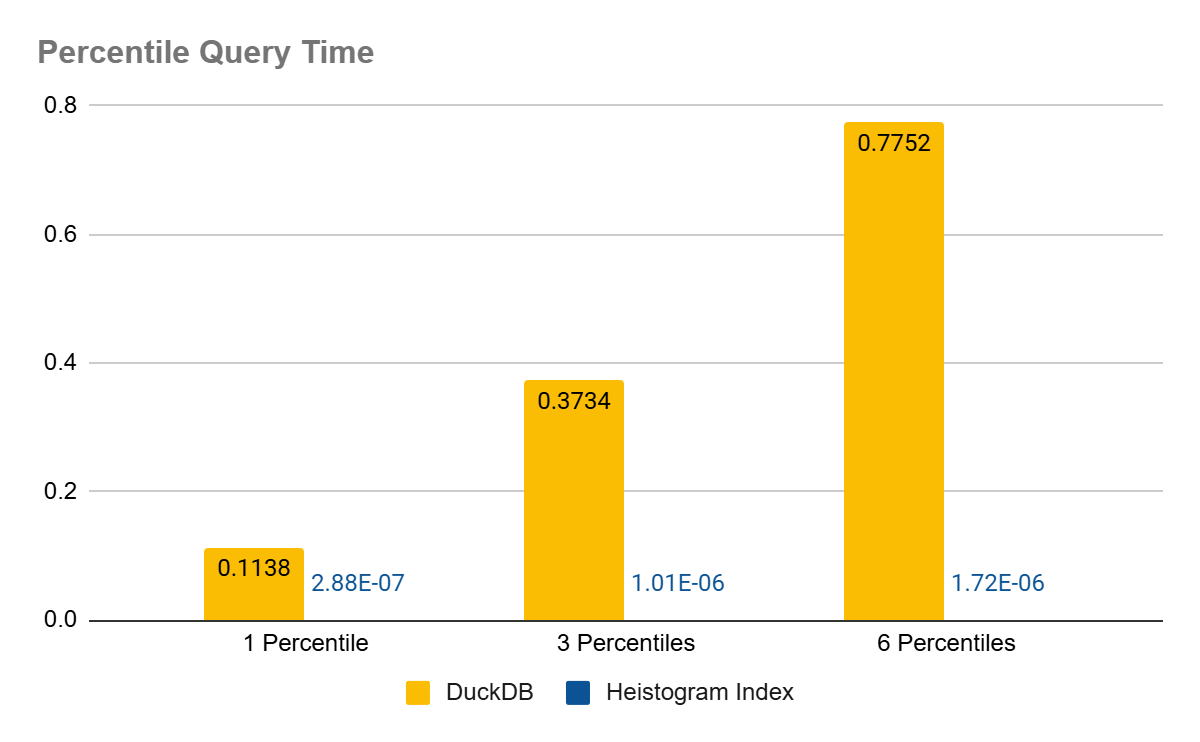
As can be seen from the chart, the query time on persisted heistograms is not even visible, I hope the data labels are clear though.
One issue with this setup though, is that it doesn’t keep up with the data. As more records are inserted into (or removed from) our samples data set the percentile queries will become less and less accurate. But we can fix that!
Take 3: Keep the Heistogram in Sync With the Data
Actually tracking changes and keeping the Heistogram in sync is pretty straightforward thanks to SQLite trigger support. Here’s what needs to be done:
CREATE TRIGGER heistogram_samples_insert AFTER INSERT ON samples
BEGIN
  UPDATE heistograms SET h = heist_add(h, NEW.sample) WHERE id = 1;
END;

CREATE TRIGGER heistogram_samples_update AFTER UPDATE OF sample ON samples
BEGIN
  UPDATE heistograms SET h = heist_remove(h, OLD.sample) WHERE id = 1;
  UPDATE heistograms SET h = heist_add(h, NEW.sample) WHERE id = 1;
END;

CREATE TRIGGER heistogram_samples_delete AFTER DELETE ON samples
BEGIN
  UPDATE heistograms SET h = heist_remove(h, OLD.sample) WHERE id = 1;
END;
These three triggers will ensure that your heistogram is always a true representation of your data set. Even if your data changes involve deletions or updates. The only draw back is that adding values individually is much slower than using the heist_group_create() or the heist_group_add() aggregate functions. Mind you, we are still talking nanoseconds per oepration, but still you will probably drop from tens of millions to only millions of operations per second.
One final issue remains, which is what if you want to get percentiles on filtered data. And here there are three options:
- Generate the heistogram on the fly like we did in the first take. Not the fastest but gets the job done
- Pre-compute the dimensions you need, you can also create the appropriate triggers to keep them in sync
- A mix of the above, pre-compute the most common dimensions and fall back to on-the-fly heistogram generation for ad-hoc queries
One thing that makes pre computing a viable strategy is how small the heistograms are. To illustrate that, I broke each of the 13M entry distributions into 10,000 heistograms (mapped on id % 10,0000). Then aggregated their sizes on disk and they were as follows:
+-------------+-------------+-----------------------------+
|  sampling   | heistograms | total heistograms size (MB) |
+-------------+-------------+-----------------------------+
| exponential | 10000       | 2.49                        |
| log_normal  | 10000       | 3.16                        |
| normal      | 10000       | 1.95                        |
| pareto      | 10000       | 3.83                        |
| random      | 10000       | 1.63                        |
+-------------+-------------+-----------------------------+
So, a 13M entry data stream when broken over 10K dimensions would still fit under 4MB. That’s quite nice! And it really makes it possible to cover a moderate number of dimensions nicely.
How to Compile heistogram_sqlite
Source is available on github and you can compile it as follows:
gcc -O3 -o heistogram heistogram_sqlite.c -lm
Conclusion
The Hiestogram SQLite extension is here, and it enables super fast percentile calculations over large data streams. Whether you create it on the fly, pre compute it or even pre compute all possible query dimensions, Heistogram is a big performance jump over what SQLite has at the moment.
It is a lean, mean, percentile calculation machine!

Leave a comment